Recommender Systems in Python: Beginner Tutorial
Recommender Systems in Python: Beginner Tutorial

Learn how to build your own recommendation engine with the help of Python, from basic models to content-based and collaborative filtering recommender systems.
Recommender systems are among the most popular applications of data science today. They are used to predict the “rating” or “preference” that a user would give to an item. Almost every major tech company has applied them in some form or the other: Amazon uses it to suggest products to customers, YouTube uses it to decide which video to play next on autoplay, and Facebook uses it to recommend pages to like and people to follow. What’s more, for some companies -think Netflix and Spotify-, the business model and its success revolves around the potency of their recommendations. In fact, Netflix even offered a million dollars in 2009 to anyone who could improve its system by 10%.
In this tutorial, you will see how to build a basic model of simple as well as content-based recommender systems. While these models will be nowhere close to the industry standard in terms of complexity, quality or accuracy, it will help you to get started with building more complex models that produce even better results.
But what are these recommender systems?
Broadly, recommender systems can be classified into 3 types:
- Simple recommenders: offer generalized recommendations to every user, based on movie popularity and/or genre. The basic idea behind this system is that movies that are more popular and critically acclaimed will have a higher probability of being liked by the average audience. IMDB Top 250 is an example of this system.
- Content-based recommenders: suggest similar items based on a particular item. This system uses item metadata, such as genre, director, description, actors, etc. for movies, to make these recommendations. The general idea behind these recommender systems is that if a person liked a particular item, he or she will also like an item that is similar to it.
- Collaborative filtering engines: these systems try to predict the rating or preference that a user would give an item-based on past ratings and preferences of other users. Collaborative filters do not require item metadata like its content-based counterparts.
Simple Recommenders
As described in the previous section, simple recommenders are basic systems that recommends the top items based on a certain metric or score. In this section, you will build a simplified clone of IMDB Top 250 Movies using metadata collected from IMDB.
The following are the steps involved:
- Decide on the metric or score to rate movies on.
- Calculate the score for every movie.
- Sort the movies based on the score and output the top results.
Before you perform any of the above steps, load your movies metadata dataset into a pandas DataFrame:
# Import Pandas
import pandas as pd

# Load Movies Metadata
metadata = pd.read_csv('../movies_dsc/data/movies_metadata.csv', low_memory=False)

# Print the first three rows
metadata.head(3)
| adult | belongs_to_collection | budget | genres | homepage | id | imdb_id | original_language | original_title | overview | … | release_date | revenue | runtime | spoken_languages | status | tagline | title | video | vote_average | vote_count | |
|---|---|---|---|---|---|---|---|---|---|---|---|---|---|---|---|---|---|---|---|---|---|
| 0 | False | {‘id’: 10194, ‘name’: ‘Toy Story Collection’, … | 30000000 | [{‘id’: 16, ‘name’: ‘Animation’}, {‘id’: 35, '… | http://toystory.disney.com/toy-story | 862 | tt0114709 | en | Toy Story | Led by Woody, Andy’s toys live happily in his … | … | 1995-10-30 | 373554033.0 | 81.0 | [{‘iso_639_1’: ‘en’, ‘name’: ‘English’}] | Released | NaN | Toy Story | False | 7.7 | 5415.0 |
| 1 | False | NaN | 65000000 | [{‘id’: 12, ‘name’: ‘Adventure’}, {‘id’: 14, '… | NaN | 8844 | tt0113497 | en | Jumanji | When siblings Judy and Peter discover an encha… | … | 1995-12-15 | 262797249.0 | 104.0 | [{‘iso_639_1’: ‘en’, ‘name’: ‘English’}, {'iso… | Released | Roll the dice and unleash the excitement! | Jumanji | False | 6.9 | 2413.0 |
| 2 | False | {‘id’: 119050, ‘name’: 'Grumpy Old Men Collect… | 0 | [{‘id’: 10749, ‘name’: ‘Romance’}, {‘id’: 35, … | NaN | 15602 | tt0113228 | en | Grumpier Old Men | A family wedding reignites the ancient feud be… | … | 1995-12-22 | 0.0 | 101.0 | [{‘iso_639_1’: ‘en’, ‘name’: ‘English’}] | Released | Still Yelling. Still Fighting. Still Ready for… | Grumpier Old Men | False | 6.5 | 92.0 |
3 rows × 24 columns
One of the most basic metrics you can think of is the rating. However, using this metric has a few caveats. For one, it does not take into consideration the popularity of a movie. Therefore, a movie with a rating of 9 from 10 voters will be considered ‘better’ than a movie with a rating of 8.9 from 10,000 voters.
On a related note, this metric will also tend to favor movies with smaller number of voters with skewed and/or extremely high ratings. As the number of voters increase, the rating of a movie regularizes and approaches towards a value that is reflective of the movie’s quality. It is more difficult to discern the quality of a movie with extremely few voters.
Taking these shortcomings into consideration, it is necessary that you come up with a weighted rating that takes into account the average rating and the number of votes it has garnered. Such a system will make sure that a movie with a 9 rating from 100,000 voters gets a (far) higher score than a YouTube Web Series with the same rating but a few hundred voters.
Since you are trying to build a clone of IMDB’s Top 250, you will use its weighted rating formula as your metric/score. Mathematically, it is represented as follows:
Weighted Rating
where,
- is the number of votes for the movie;
- is the minimum votes required to be listed in the chart;
- is the average rating of the movie; And
- is the mean vote across the whole report
You already have the values to v (vote_count) and R (vote_average) for each movie in the dataset. It is also possible to directly calculate C from this data.
What you need to determine is an appropriate value for m, the minimum votes required to be listed in the chart. There is no right value for m. You can view it as a preliminary negative filter that ignores movies which have less than a certain number of votes. The selectivity of your filter is up to your discretion.
In this case, you will use the 90th percentile as your cutoff. In other words, for a movie to feature in the charts, it must have more votes than at least 90% of the movies in the list. (On the other hand, if you had chosen the 75th percentile, you would have considered the top 25% of the movies in terms of the number of votes garnered. As the percentile decreases, the number of movies considered increases. Feel free to play with this value and observe the changes in your final chart).
As a first step, let’s calculate the value of C, the mean rating across all movies:
# Calculate C
C = metadata['vote_average'].mean()
print(C)
5.61820721513
The average rating of a movie on IMDB is around 5.6, on a scale of 10.
Next, let’s calculate the number of votes, m, received by a movie in the 90th percentile. The pandas library makes this task extremely trivial using the .quantile() method of a pandas Series:
# Calculate the minimum number of votes required to be in the chart, m
m = metadata['vote_count'].quantile(0.90)
print(m)
160.0
Next, you can filter the movies that qualify for the chart, based on their vote counts:
# Filter out all qualified movies into a new DataFrame
q_movies = metadata.copy().loc[metadata['vote_count'] >= m]
q_movies.shape
(4555, 24)
You use the .copy() method to ensure that the new q_movies DataFrame created is independent of your original metadata DataFrame. In other words, any changes made to the q_movies DataFrame does not affect the metadata.
You see that there are 4555 movies which qualify to be in this list. Now, you need to calculate your metric for each qualified movie. To do this, you will define a function, weighted_rating() and define a new feature score, of which you’ll calculate the value by applying this function to your DataFrame of qualified movies:
# Function that computes the weighted rating of each movie
def weighted_rating(x, m=m, C=C):
    v = x['vote_count']
    R = x['vote_average']
    # Calculation based on the IMDB formula
    return (v/(v+m) * R) + (m/(m+v) * C)
# Define a new feature 'score' and calculate its value with `weighted_rating()`
q_movies['score'] = q_movies.apply(weighted_rating, axis=1)
Finally, let’s sort the DataFrame based on the score feature and output the title, vote count, vote average and weighted rating or score of the top 15 movies.
#Sort movies based on score calculated above
q_movies = q_movies.sort_values('score', ascending=False)

#Print the top 15 movies
q_movies[['title', 'vote_count', 'vote_average', 'score']].head(15)
| title | vote_count | vote_average | score | |
|---|---|---|---|---|
| 314 | The Shawshank Redemption | 8358.0 | 8.5 | 8.445869 |
| 834 | The Godfather | 6024.0 | 8.5 | 8.425439 |
| 10309 | Dilwale Dulhania Le Jayenge | 661.0 | 9.1 | 8.421453 |
| 12481 | The Dark Knight | 12269.0 | 8.3 | 8.265477 |
| 2843 | Fight Club | 9678.0 | 8.3 | 8.256385 |
| 292 | Pulp Fiction | 8670.0 | 8.3 | 8.251406 |
| 522 | Schindler’s List | 4436.0 | 8.3 | 8.206639 |
| 23673 | Whiplash | 4376.0 | 8.3 | 8.205404 |
| 5481 | Spirited Away | 3968.0 | 8.3 | 8.196055 |
| 2211 | Life Is Beautiful | 3643.0 | 8.3 | 8.187171 |
| 1178 | The Godfather: Part II | 3418.0 | 8.3 | 8.180076 |
| 1152 | One Flew Over the Cuckoo’s Nest | 3001.0 | 8.3 | 8.164256 |
| 351 | Forrest Gump | 8147.0 | 8.2 | 8.150272 |
| 1154 | The Empire Strikes Back | 5998.0 | 8.2 | 8.132919 |
| 1176 | Psycho | 2405.0 | 8.3 | 8.132715 |
You see that the chart has a lot of movies in common with the IMDB Top 250 chart: for example, your top two movies, “Shawshank Redemption” and “The Godfather”, are the same as IMDB.
Content-Based Recommender in Python
Plot Description Based Recommender
In this section, you will try to build a system that recommends movies that are similar to a particular movie. More specifically, you will compute pairwise similarity scores for all movies based on their plot descriptions and recommend movies based on that similarity score.
The plot description is available to you as the overview feature in your metadata dataset. Let’s inspect the plots of a few movies:
#Print plot overviews of the first 5 movies.
metadata['overview'].head()
0    Led by Woody, Andy's toys live happily in his ...
1    When siblings Judy and Peter discover an encha...
2    A family wedding reignites the ancient feud be...
3    Cheated on, mistreated and stepped on, the wom...
4    Just when George Banks has recovered from his ...
Name: overview, dtype: object
In its current form, it is not possible to compute the similarity between any two overviews. To do this, you need to compute the word vectors of each overview or document, as it will be called from now on.
You will compute Term Frequency-Inverse Document Frequency (TF-IDF) vectors for each document. This will give you a matrix where each column represents a word in the overview vocabulary (all the words that appear in at least one document) and each column represents a movie, as before.
In its essence, the TF-IDF score is the frequency of a word occurring in a document, down-weighted by the number of documents in which it occurs. This is done to reduce the importance of words that occur frequently in plot overviews and therefore, their significance in computing the final similarity score.
Fortunately, scikit-learn gives you a built-in TfIdfVectorizer class that produces the TF-IDF matrix in a couple of lines.
#Import TfIdfVectorizer from scikit-learn
from sklearn.feature_extraction.text import TfidfVectorizer

#Define a TF-IDF Vectorizer Object. Remove all english stop words such as 'the', 'a'
tfidf = TfidfVectorizer(stop_words='english')

#Replace NaN with an empty string
metadata['overview'] = metadata['overview'].fillna('')

#Construct the required TF-IDF matrix by fitting and transforming the data
tfidf_matrix = tfidf.fit_transform(metadata['overview'])

#Output the shape of tfidf_matrix
tfidf_matrix.shape
(45466, 75827)
You see that over 75,000 different words were used to describe the 45,000 movies in your dataset.
With this matrix in hand, you can now compute a similarity score. There are several candidates for this; such as the euclidean, the Pearson and the cosine similarity scores. Again, there is no right answer to which score is the best. Different scores work well in different scenarios and it is often a good idea to experiment with different metrics.
You will be using the cosine similarity to calculate a numeric quantity that denotes the similarity between two movies. You use the cosine similarity score since it is independent of magnitude and is relatively easy and fast to calculate (especially when used in conjunction with TF-IDF scores, which will be explained later). Mathematically, it is defined as follows:
Since you have used the TF-IDF vectorizer, calculating the dot product will directly give you the cosine similarity score. Therefore, you will use sklearn's linear_kernel() instead of cosine_similarities() since it is faster.
# Import linear_kernel
from sklearn.metrics.pairwise import linear_kernel

# Compute the cosine similarity matrix
cosine_sim = linear_kernel(tfidf_matrix, tfidf_matrix)
You’re going to define a function that takes in a movie title as an input and outputs a list of the 10 most similar movies. Firstly, for this, you need a reverse mapping of movie titles and DataFrame indices. In other words, you need a mechanism to identify the index of a movie in your metadata DataFrame, given its title.
#Construct a reverse map of indices and movie titles
indices = pd.Series(metadata.index, index=metadata['title']).drop_duplicates()
You are now in a good position to define your recommendation function. These are the following steps you’ll follow:
- Get the index of the movie given its title.
- Get the list of cosine similarity scores for that particular movie with all movies. Convert it into a list of tuples where the first element is its position and the second is the similarity score.
- Sort the aforementioned list of tuples based on the similarity scores; that is, the second element.
- Get the top 10 elements of this list. Ignore the first element as it refers to self (the movie most similar to a particular movie is the movie itself).
- Return the titles corresponding to the indices of the top elements.
# Function that takes in movie title as input and outputs most similar movies
def get_recommendations(title, cosine_sim=cosine_sim):
    # Get the index of the movie that matches the title
    idx = indices[title]

    # Get the pairwsie similarity scores of all movies with that movie
    sim_scores = list(enumerate(cosine_sim[idx]))

    # Sort the movies based on the similarity scores
    sim_scores = sorted(sim_scores, key=lambda x: x[1], reverse=True)

    # Get the scores of the 10 most similar movies
    sim_scores = sim_scores[1:11]

    # Get the movie indices
    movie_indices = [i[0] for i in sim_scores]

    # Return the top 10 most similar movies
    return metadata['title'].iloc[movie_indices]
get_recommendations('The Dark Knight Rises')
12481                                      The Dark Knight
150                                         Batman Forever
1328                                        Batman Returns
15511                           Batman: Under the Red Hood
585                                                 Batman
21194    Batman Unmasked: The Psychology of the Dark Kn...
9230                    Batman Beyond: Return of the Joker
18035                                     Batman: Year One
19792              Batman: The Dark Knight Returns, Part 1
3095                          Batman: Mask of the Phantasm
Name: title, dtype: object
get_recommendations('The Godfather')
1178               The Godfather: Part II
44030    The Godfather Trilogy: 1972-1990
1914              The Godfather: Part III
23126                          Blood Ties
11297                    Household Saints
34717                   Start Liquidation
10821                            Election
38030            A Mother Should Be Loved
17729                   Short Sharp Shock
26293                  Beck 28 - Familjen
Name: title, dtype: object
You see that, while your system has done a decent job of finding movies with similar plot descriptions, the quality of recommendations is not that great. “The Dark Knight Rises” returns all Batman movies while it more likely that the people who liked that movie are more inclined to enjoy other Christopher Nolan movies. This is something that cannot be captured by your present system.
Credits, Genres and Keywords Based Recommender
It goes without saying that the quality of your recommender would be increased with the usage of better metadata. That is exactly what you are going to do in this section. You are going to build a recommender based on the following metadata: the 3 top actors, the director, related genres and the movie plot keywords.
The keywords, cast and crew data is not available in your current dataset so the first step would be to load and merge them into your main DataFrame.
# Load keywords and credits
credits = pd.read_csv('../movies_dsc/data/credits.csv')
keywords = pd.read_csv('../movies_dsc/data/keywords.csv')

# Remove rows with bad IDs.
metadata = metadata.drop([19730, 29503, 35587])

# Convert IDs to int. Required for merging
keywords['id'] = keywords['id'].astype('int')
credits['id'] = credits['id'].astype('int')
metadata['id'] = metadata['id'].astype('int')

# Merge keywords and credits into your main metadata dataframe
metadata = metadata.merge(credits, on='id')
metadata = metadata.merge(keywords, on='id')
# Print the first two movies of your newly merged metadata
metadata.head(2)
| adult | belongs_to_collection | budget | genres | homepage | id | imdb_id | original_language | original_title | overview | … | spoken_languages | status | tagline | title | video | vote_average | vote_count | cast | crew | keywords | |
|---|---|---|---|---|---|---|---|---|---|---|---|---|---|---|---|---|---|---|---|---|---|
| 0 | False | {‘id’: 10194, ‘name’: ‘Toy Story Collection’, … | 30000000 | [{‘id’: 16, ‘name’: ‘Animation’}, {‘id’: 35, '… | http://toystory.disney.com/toy-story | 862 | tt0114709 | en | Toy Story | Led by Woody, Andy’s toys live happily in his … | … | [{‘iso_639_1’: ‘en’, ‘name’: ‘English’}] | Released | NaN | Toy Story | False | 7.7 | 5415.0 | [{‘cast_id’: 14, ‘character’: ‘Woody (voice)’,… | [{‘credit_id’: ‘52fe4284c3a36847f8024f49’, 'de… | [{‘id’: 931, ‘name’: ‘jealousy’}, {‘id’: 4290,… |
| 1 | False | NaN | 65000000 | [{‘id’: 12, ‘name’: ‘Adventure’}, {‘id’: 14, '… | NaN | 8844 | tt0113497 | en | Jumanji | When siblings Judy and Peter discover an encha… | … | [{‘iso_639_1’: ‘en’, ‘name’: ‘English’}, {'iso… | Released | Roll the dice and unleash the excitement! | Jumanji | False | 6.9 | 2413.0 | [{‘cast_id’: 1, ‘character’: ‘Alan Parrish’, '… | [{‘credit_id’: ‘52fe44bfc3a36847f80a7cd1’, 'de… | [{‘id’: 10090, ‘name’: ‘board game’}, {‘id’: 1… |
2 rows × 27 columns
From your new features, cast, crew and keywords, you need to extract the three most important actors, the director and the keywords associated with that movie. Right now, your data is present in the form of “stringified” lists. You need to convert them into a form that is usable for you.
# Parse the stringified features into their corresponding python objects
from ast import literal_eval

features = ['cast', 'crew', 'keywords', 'genres']
for feature in features:
    metadata[feature] = metadata[feature].apply(literal_eval)
Next, you write functions that will help you to extract the required information from each feature. First, you’ll import the NumPy package to get access to its NaN constant. Next, you can use it to write the get_director() function:
# Import Numpy
import numpy as np
# Get the director's name from the crew feature. If director is not listed, return NaN
def get_director(x):
    for i in x:
        if i['job'] == 'Director':
            return i['name']
    return np.nan
# Returns the list top 3 elements or entire list; whichever is more.
def get_list(x):
    if isinstance(x, list):
        names = [i['name'] for i in x]
        #Check if more than 3 elements exist. If yes, return only first three. If no, return entire list.
        if len(names) > 3:
            names = names[:3]
        return names

    #Return empty list in case of missing/malformed data
    return []
# Define new director, cast, genres and keywords features that are in a suitable form.
metadata['director'] = metadata['crew'].apply(get_director)

features = ['cast', 'keywords', 'genres']
for feature in features:
    metadata[feature] = metadata[feature].apply(get_list)
# Print the new features of the first 3 films
metadata[['title', 'cast', 'director', 'keywords', 'genres']].head(3)
| title | cast | director | keywords | genres | |
|---|---|---|---|---|---|
| 0 | Toy Story | [Tom Hanks, Tim Allen, Don Rickles] | John Lasseter | [jealousy, toy, boy] | [Animation, Comedy, Family] |
| 1 | Jumanji | [Robin Williams, Jonathan Hyde, Kirsten Dunst] | Joe Johnston | [board game, disappearance, based on children’… | [Adventure, Fantasy, Family] |
| 2 | Grumpier Old Men | [Walter Matthau, Jack Lemmon, Ann-Margret] | Howard Deutch | [fishing, best friend, duringcreditsstinger] | [Romance, Comedy] |
The next step would be to convert the names and keyword instances into lowercase and strip all the spaces between them. This is done so that your vectorizer doesn’t count the Johnny of “Johnny Depp” and “Johnny Galecki” as the same. After this processing step, the aforementioned actors will be represented as “johnnydepp” and “johnnygalecki” and will be distinct to your vectorizer.
# Function to convert all strings to lower case and strip names of spaces
def clean_data(x):
    if isinstance(x, list):
        return [str.lower(i.replace(" ", "")) for i in x]
    else:
        #Check if director exists. If not, return empty string
        if isinstance(x, str):
            return str.lower(x.replace(" ", ""))
        else:
            return ''
# Apply clean_data function to your features.
features = ['cast', 'keywords', 'director', 'genres']

for feature in features:
    metadata[feature] = metadata[feature].apply(clean_data)
You are now in a position to create your “metadata soup”, which is a string that contains all the metadata that you want to feed to your vectorizer (namely actors, director and keywords).
def create_soup(x):
    return ' '.join(x['keywords']) + ' ' + ' '.join(x['cast']) + ' ' + x['director'] + ' ' + ' '.join(x['genres'])
# Create a new soup feature
metadata['soup'] = metadata.apply(create_soup, axis=1)
The next steps are the same as what you did with your plot description based recommender. One important difference is that you use the CountVectorizer() instead of TF-IDF. This is because you do not want to down-weight the presence of an actor/director if he or she has acted or directed in relatively more movies. It doesn’t make much intuitive sense.
# Import CountVectorizer and create the count matrix
from sklearn.feature_extraction.text import CountVectorizer

count = CountVectorizer(stop_words='english')
count_matrix = count.fit_transform(metadata['soup'])
# Compute the Cosine Similarity matrix based on the count_matrix
from sklearn.metrics.pairwise import cosine_similarity

cosine_sim2 = cosine_similarity(count_matrix, count_matrix)
# Reset index of your main DataFrame and construct reverse mapping as before
metadata = metadata.reset_index()
indices = pd.Series(metadata.index, index=metadata['title'])
You can now reuse your get_recommendations() function by passing in the new cosine_sim2 matrix as your second argument.
get_recommendations('The Dark Knight Rises', cosine_sim2)
12589      The Dark Knight
10210        Batman Begins
9311                Shiner
9874       Amongst Friends
7772              Mitchell
516      Romeo Is Bleeding
11463         The Prestige
24090            Quicksand
25038             Deadfall
41063                 Sara
Name: title, dtype: object
get_recommendations('The Godfather', cosine_sim2)
1934            The Godfather: Part III
1199             The Godfather: Part II
15609                   The Rain People
18940                         Last Exit
34488                              Rege
35802            Manuscripts Don't Burn
35803            Manuscripts Don't Burn
8001     The Night of the Following Day
18261                 The Son of No One
28683            In the Name of the Law
Name: title, dtype: object
You see that your recommender has been successful in capturing more information due to more metadata and has given you (arguably) better recommendations. There are, of course, numerous ways of playing with this system in order to improve recommendations.
Some suggestions:
- Introduce a popularity filter: this recommender would take the list of the 30 most similar movies, calculate the weighted ratings (using the IMDB formula from above), sort movies based on this rating and return the top 10 movies.
- Other crew members: other crew member names, such as screenwriters and producers, could also be included.
- Increasing weight of the director: to give more weight to the director, he or she could be mentioned multiple times in the soup to increase the similarity scores of movies with the same director.
You can find these ideas implemented in this notebook.
Collaborative Filtering with Python
In this tutorial, you have learnt how to build your very own Simple and Content Based Movie Recommender Systems. There is also another extremely popular type of recommender known as collaborative filters.
Collaborative filters can further be classified into two types:
- User-based Filtering: these systems recommend products to a user that similar users have liked. For example, let’s say Alice and Bob have a similar interest in books (that is, they largely like and dislike the same books). Now, let’s say a new book has been launched into the market and Alice has read and loved it. It is therefore, highly likely that Bob will like it too and therefore, the system recommends this book to Bob.
- Item-based Filtering: these systems are extremely similar to the content recommendation engine that you built. These systems identify similar items based on how people have rated it in the past. For example, if Alice, Bob and Eve have given 5 stars to The Lord of the Rings and The Hobbit, the system identifies the items as similar. Therefore, if someone buys The Lord of the Rings, the system also recommends The Hobbit to him or her.
You will not be building these systems in this tutorial but you are already familiar with most of the ideas required to do so. A good place to start with collaborative filters is by examining the MovieLens dataset, which can be found here.
Conclusion
In this tutorial, you have covered how to build simple as well as content-based recommenders. Hopefully, you are now in a good position to make improvements on the basic systems you built and experiment with other kinds of recommenders (such as collaborative filters). I hope you had as much fun reading this as I had writing. Happy recommending!


来源:网络
智能推荐
推荐系统公平性之流行度偏差(fairness in recommender systems -- popularity bias)
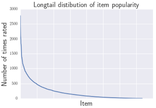
主要参考论文:《The Unfairness of Popularity Bias in Recommendation》 RMSE@RecSys 2019 流行度偏差是什么 先定义流行物品和非流行物品。下图是(Movielens 1M)数据集中物品的评分情况。 图的横坐标表示不同物品,纵坐标表示物品的评分次数。可以看出只有少部分物品得到了很多的评分,大部分曲线尾部的物品都只有少量的评分,我们也把这...
博文翻译:Tackling the Cold Start Problem in Recommender Systems
博文地址:Tackling the Cold Start Problem in Recommender Systems 题目:Tackling the Cold Start Problem in Recommender Systems / 解决推荐系统中的冷启动问题 作者:Kojin Oshiba 当我在Wish进行机器学习实习时,我要解决推荐系统中的一个常见问题“冷启动...

Complete Java Collection tutorial for the beginner
http://www.jitendrazaa.com/blog/java/complete-java-collection-tutorial-for-the-beginner/ Complete Java Collection tutorial for the beginner Collection represents the group of objects. Depending on the...
[论文阅读] 对话式推荐系统的进展与挑战:综述(Advances and Challenges in Conversational Recommender Systems: ASurvey)-03
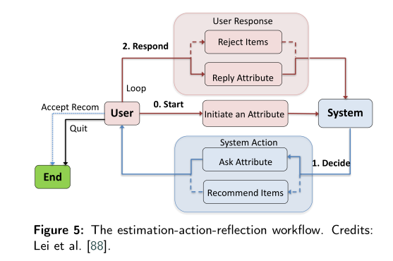
0. 序言 本文接续上一篇,主要讲在发展CRS中主要遇到的另一个挑战 multi-turn conversational strategy 多轮对话策略。 1. Multi-turn Conversational Strategies for CRSs 问题驱动法侧重于“问什么”(What to ask)的问题,本节讨论的多轮对话...
[论文阅读] 对话式推荐系统的进展与挑战:综述(Advances and Challenges in Conversational Recommender Systems: ASurvey)-06
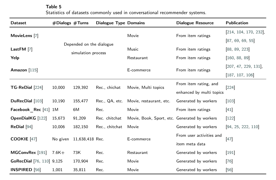
0. 序言 本文介绍CRS的最后一个主要挑战:Evaluation and User Simulation 评估和用户模拟 1. Evaluation 常见数据集如下,大部分研究采用基于对通用数据模拟得到的对话数据进行处理。部分采用众包平台进行真实对话收集。CRS评估开源工具:https://github.com/RUCAIBox/CRSL...
猜你喜欢

Wide & Deep Learning for Recommender Systems
ABSTRACT 通过特征的向量积(cross-product)对特征交叉的记忆具有可解释性,而泛化又需要更多的特征工程。而DNN通过对稀疏特征学习低维稠密的embedding表示对未出现的特征组合具有良好的泛化性能。但是,当用户物品关系比较稀疏,维度又比较高时,DNN容易过度泛化,推荐一些不相干的物品。文中提出Wide&Deep 学习,同时训练wide 部分和dnn,将记忆性和泛化性结合...
原型对象,原型链
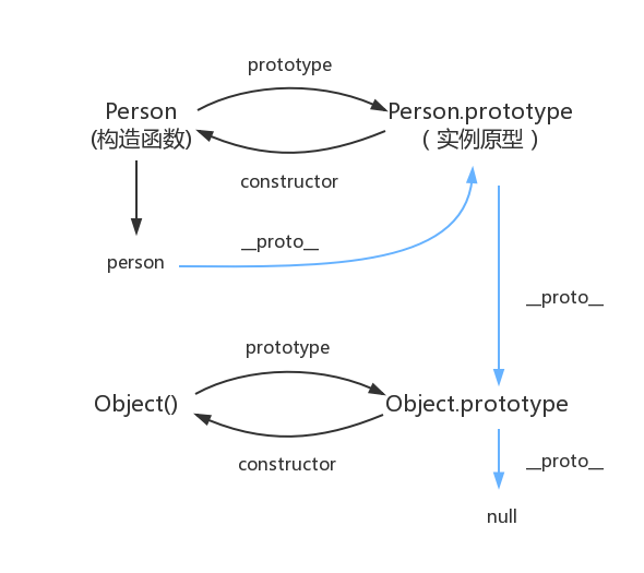
函数都有prototype属性,它指向原型对象。 实例对象有__proto__属性,它指向对象原型 每一个原型对象都有constructor输赢,指向构造函数,每一个原型对象又具有__proto__属性,这个指向Object.prototype.在这里插入图片描述...

Node 调用 dubbo 服务的探索及实践
2.Dubbo简介 2.1 什么是dubbo Dubbo是一款高性能、轻量级的开源Java RPC框架,它提供了三大核心能力:面向接口的远程方法调用,智能容错和负载均衡,以及服务自动注册和发现。 2.2 流程图 Provider : 暴露服务的服务提供方。 Consumer : 调用远程服务的服务消费方。 Registry : 服务注册与发现的注册中心。 Monito...

mysql总结
mysql基础入门的总结 关于数据库: 数据库是软件开发人员要掌握的基本工具,软件的运行的过程就是操作数据的过程,数据库中的数据无非就是几个操作:增-删-查-改。 Mysql安装完成后,需要配置变量环境,找到配置路径path,然后把mysql安装目录bin文件导入就可以了。 然后运行cm...
adb及monkey常用命令
adb常用命令: 查看手机是否连接:adb devices 连接设备:adb connect 设备ip:端口号 若有连接多个设备需指明设备ip及端口号 安装APP:adb install [-r] 包名 -r表示覆盖安装,首次安装可省略 卸载APP:adb uninstall 包名 列出设备中所有应用包名:adb shell pm list packages ...
问答精选
Correctly formatting GCM notifications?
I'm currently trying out the google cloud messaging service with its sample application "Guestbook." https://developers.google.com/cloud/samples/mbs/ I'm attempting to send notifications tha...
Are there any performance benefits of using Asynchronous functions over Synchronous in Node Js?
Now I came across an article that distinguishes between an Asynchronous function and Synchronous functions. From my understanding of the different examples and explanations, synchronous functions are ...
Python: Costing calculator output
Good day all I'm busy creating a small costing calculator for the signage department. I'm not getting the calculator to output the amount. Brief Description: You enter the height and width and then wh...
Flask-SQLAlchemy - model has no attribute 'foreign_keys'
I have 3 models created with Flask-SQLalchemy: User, Role, UserRole role.py: user.py: user_role.py: If I try (in the console) to get all users via User.query.all() I get AttributeError: 'NoneType' obj...
Seeding many PRNGs, then having to seed them again, what is a good quality approach?
I have many particles that follow an stochastic process in parallel. For each particle, there is a PRNG associated to it. The simulation must go through many repetitions to get average results. For ea...
相关问题
- 如何在Python-Beginner中循环
- Rails Beginner - which controller to put functions in?
- Would developing in different CMS systems be beneficial?
- Boost.Python Tutorial在Ubuntu 10.04
- Eclipse as an IDE - What do you find missing as a beginner in Java?
- Python源代码转换为带有Sparx Systems Enterprise Architect的UML图表
- PowerBuilder beginner question
- Visual Basic Beginner ..substrings
- Java Beginner协调界外
- Docker-Compose Tutorial不起作用“Python:无法打开文件'manage.py”
相关文章
- Multiple Objective Optimization in Recommender Systems
- Graph Neural Networks in Recommender Systems综述
- Zipline Beginner Tutorial
- 《Wide and deep learning in Recommender Systems》论文阅读笔记
- 《DropoutNet: Addressing Cold Start in Recommender Systems》论文阅读笔记
- Paper Notes: Graph Neural Networks in Recommender Systems - A Survey
- Graph Neural Networks in Recommender Systems综述(文章搬运)
- Graph Neural Networks in Recommender Systems: A Survey
- 机器学习-Recommender Systems
- 推荐系统(Recommender Systems)
热门文章
推荐文章
相关标签
推荐问答
- ShareActionProvider with background processing
- gridview changing position automatically when notifiedDatasetChangedCalled?
- How to efficiently fill-in a structure with vectors?
- when i exit from node js, i just cant give command in my terminal
- How to upload an image with Spray?
- Edit my message before posting in Twitter with Twitter API and PHP
- Using css style selector in JQuery not working?
- Can Html.Display/Html.DisplayFor/Html.DisplayForModel work with a DataTable?
- What does <?!= mean in Google Apps Script?
- Python/Linux - Manually installing httplib2 as a non-root user